Quick demo

# remotes::install_github("PengSU517/regcell")
library(regcell)
library(tidyverse)

A simulated dataset

We generate a dataset that incorporates a design matrix with 200 observations and 50 variables. The contamination rate is set to 5%, and the scale of residuals is fixed at 3, while retaining the default values for other settings.

set.seed(1234)
dat = regcell::genevar(n = 200, p = 50, e = 0.05, sigma = 3) 

y = dat$y
x = dat$x

Outlier detection

Detect outliers using DDC (Rousseeuw & Van Den Bossche, 2018).

fit1 <- cellWise::DDC(x)
#>  
#>  The input data has 200 rows and 50 columns.
p1 = regcell::newcellmap(fit1$stdResid, columnlabels = c(dim(x)[2],rep(" ",dim(x)[2]-2),1), rowlabels = c(dim(x)[1],rep(" ",dim(x)[1]-2),1), columnangle = 0,
        rowtitle = "Observations", columntitle = "Variables", sizetitles = 2,adjustrowlabels = 0.5, adjustcolumnlabels = 0.5)+
   theme(axis.text.x = element_text(size = 12),
        axis.text.y = element_text(size = 12),
        axis.title.x = element_text(size = 14),
        axis.title.y = element_text(size = 14),
        legend.title = element_text(size=14), #change legend title font size
        legend.text = element_text(size=12)) +
  coord_flip()
p1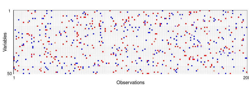

Figure 1: Outlier cell map of the generated dataset. Cells are flagged as outlying if the observed and predicted values differ too much. Most cells are blank, showing they are not detected as outliers. A red cell means the observed value is significantly higher than the predicted value, and a blue cell means the observed value is significantly lower.

Model training

We establish a training set and a testing set. Subsequently, we employ the training set to fit models and assess prediction errors by evaluating their performance on the testing set.

set.seed(1234)
inTrain <- caret::createDataPartition(y, p = 0.7)[[1]]


ytrain = y[inTrain]
xtrain = x[inTrain,]

ytest = y[-inTrain]
xtest = x[-inTrain,]

set.seed(1234)
#fit a model using CR-Lasso
fit0 = sregcell_std(ytrain,xtrain)
res = ytest - fit0$intercept_hat - xtest%*%fit0$betahat

#fit a model using RLars
fit1 = Rlars(ytrain,xtrain)
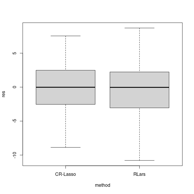
res2 = ytest - fit1$betahat[1] - xtest%*%fit1$betahat[-1]

The figure below illustrates the distribution of prediction errors derived from the test set.

df = data.frame(res = c(res, res2), 
                method = c(rep("CR-Lasso", length(res)),rep("RLars", length(res)) ))
boxplot(res~method, outline = FALSE, data = df)

Rousseeuw, P. J., & Van Den Bossche, W. (2018). Detecting deviating data cells. Technometrics, 60, 135–145.